저번 시간에 review 한 DCGAN 논문의 code reivew입니다.
DCGAN 논문에 대한 세부사항이 궁금하시다면, 다음 주소에서 확인하실 수 있습니다.
4. Unsupervised Representation learning with Deep Convolutional Generative Adversarial Networks(DCGAN) - paper review
오늘은 Generative Adversarial networks에 Convolutional neural network를 섞은 모델인 DCGAN에 대해서 리뷰를 해보겠습니다. original paper : arxiv.org/abs/1511.06434 Unsupervised Representation Learning..
cumulu-s.tistory.com
이번 글에서는 DCGAN 논문에 나온 정보를 바탕으로, 실제로 DCGAN 모델을 짜 보고 결과를 확인해보겠습니다.
시작합니다.
from torch.utils.tensorboard import SummaryWriter
import os
import random
import torch
import torch.nn as nn
import torch.optim as optim
import torch.utils.data
import torchvision.datasets
import torchvision.transforms as transforms
import torchvision.utils as vutils
import datetime
import shutil
import matplotlib.pyplot as plt
import numpy as np
from torch.autograd import Variable
import math
from tqdm.auto import tqdm
먼저 필요한 패키지들을 불러옵니다.
current_time = datetime.datetime.now() + datetime.timedelta(hours= 9)
current_time = current_time.strftime('%Y-%m-%d-%H:%M')

saved_loc = os.path.join('/content/drive/MyDrive/DCGAN_Result', current_time)
if os.path.exists(saved_loc):
    shutil.rmtree(saved_loc)
os.mkdir(saved_loc)

image_loc = os.path.join(saved_loc, "images")
os.mkdir(image_loc)
weight_loc = os.path.join(saved_loc, "weights")
os.mkdir(weight_loc)

print("결과 저장 위치: ", saved_loc)
print("이미지 저장 위치: ", image_loc)
print("가중치 저장 위치: ", weight_loc)

writer = SummaryWriter(saved_loc)

random.seed(999)
torch.manual_seed(999)
current_time은 Google colab을 사용하면 시간이 9시간 밀려서 현재 시간을 찍기 위해 만들어진 것이고,
os.mkdir를 이용해서 결과를 저장할 폴더를 만들어줍니다.
SummaryWriter는 tensorboard에 학습 결과를 찍기 위해 만들어줍니다.
결과를 다시 그대로 볼 수 있도록, random seed와 manual seed를 따로 주었습니다.
transformation = transforms.Compose([
        transforms.Resize(64),
        transforms.ToTensor(),
        transforms.Normalize((0.5,), (0.5,)),
    ])


train_dataset = torchvision.datasets.FashionMNIST(root = '/content/drive/MyDrive/Fashion_MNIST', train = True, download = True,
                                            transform = transformation)

print("dataset size: ", len(train_dataset))

trainloader = torch.utils.data.DataLoader(train_dataset, batch_size = BATCH_SIZE, shuffle = True, num_workers = 2)


USE_CUDA = torch.cuda.is_available()
device = torch.device("cuda" if USE_CUDA else "cpu")
데이터셋으로는 FashionMNIST를 들고 오고, 논문에서 64x64로 실험을 했으므로 이를 그대로 사용하기 위해 Resize를 통해서 64x64의 이미지로 만들어줍니다. (제 Github에는 32x32로 실험된 결과들도 있습니다.)
USE_CUDA = torch.cuda.is_available()
device = torch.device("cuda" if USE_CUDA else "cpu")
저는 GPU 연산을 사용하기 때문에, cuda 설정을 해줍니다.
# Generator
class Generator(torch.nn.Module):
def __init__(self, channels):
super().__init__()
# Filters [1024, 512, 256, 128]
# Input_dim = 100
# Output_dim = C (number of channels)
self.main_module = nn.Sequential(
# Z latent vector 100
nn.ConvTranspose2d(in_channels=100, out_channels=1024, kernel_size=4, stride=1, padding=0),
nn.BatchNorm2d(num_features=1024),
nn.ReLU(True),
# State (1024x4x4)
nn.ConvTranspose2d(in_channels=1024, out_channels=512, kernel_size=4, stride=2, padding=1),
nn.BatchNorm2d(num_features=512),
nn.ReLU(True),
# State (512x8x8)
nn.ConvTranspose2d(in_channels=512, out_channels=256, kernel_size=4, stride=2, padding=1),
nn.BatchNorm2d(num_features=256),
nn.ReLU(True),
# State (256x16x16)
nn.ConvTranspose2d(in_channels=256, out_channels=128, kernel_size=4, stride=2, padding=1),
nn.BatchNorm2d(num_features=128),
nn.ReLU(True),
# State (128x32x32)
nn.ConvTranspose2d(in_channels=128, out_channels=channels, kernel_size=4, stride=2, padding=1))
# output of main module --> Image (Cx64x64)
self.output = nn.Tanh()
def forward(self, x):
x = self.main_module(x)
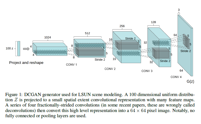
return self.output(x)다음으로는 Generator model을 살펴보겠습니다.
이는 논문에 나온 구조를 그대로 따라서 만든 거라고 보시면 되겠습니다.
# Discriminator
class Discriminator(torch.nn.Module):
    def __init__(self, channels):
        super().__init__()
        # Filters [128, 256, 512, 1024]
        # Input_dim = channels (Cx64x64)
        # Output_dim = 1
        self.main_module = nn.Sequential(
            # Image (Cx64x64)
            nn.Conv2d(in_channels=channels, out_channels=128, kernel_size=4, stride=2, padding=1),
            nn.LeakyReLU(0.2, inplace=True),

            # State (128x32x32)
            nn.Conv2d(in_channels=128, out_channels=256, kernel_size=4, stride=2, padding=1),
            nn.BatchNorm2d(256),
            nn.LeakyReLU(0.2, inplace=True),

            # State (256x16x16)
            nn.Conv2d(in_channels=256, out_channels=512, kernel_size=4, stride=2, padding=1),
            nn.BatchNorm2d(512),
            nn.LeakyReLU(0.2, inplace=True),

            # State (512x8x8)
            nn.Conv2d(in_channels=512, out_channels=1024, kernel_size=4, stride=2, padding=1),
            nn.BatchNorm2d(1024),
            nn.LeakyReLU(0.2, inplace=True))
            # outptut of main module --> State (1024x4x4)

        self.output = nn.Sequential(
            nn.Conv2d(in_channels=1024, out_channels=1, kernel_size=4, stride=1, padding=0),
            # Output 1
            nn.Sigmoid())

    def forward(self, x):
        x = self.main_module(x)
        return self.output(x)
다음으로는 discriminator 구조를 살펴보겠습니다.
이는 generator의 구조를 그대로 가져오되, 반대로 만든 거라고 생각하시면 되겠습니다.
즉, (batch, 1, 64, 64)의 이미지를 받아서 convolution 연산을 거듭하면서 channel은 늘리고 가로 세로 사이즈는 2배씩 줄입니다.
마지막으로는 (batch, 1024, 4, 4)에서 (batch, 1, 1, 1) 형태로 만들어주면서 input으로 받은 이미지가 진짜인지 가짜인지에 대한 값이 나오도록 만들어줍니다. 그래서 맨 마지막의 activation function은 Sigmoid가 사용됩니다.
그리고 이전 모델과 다른 점이라면, layer 사이에 사용되는 activation function은 LeakyReLU를 사용해줍니다. 이는 논문에서 언급된 사항이죠.
마찬가지로 BatchNorm은 layer마다 꼭 사용해줘야 하고요.
netG = Generator(1).to(device)
netD = Discriminator(1).to(device)

criterion = nn.BCELoss()

# To see fixed noise vector's change
fixed_noise = torch.randn(16, 100, 1, 1, device=device)
real_label = 1
fake_label = 0

# setup optimizer
optimizerD = optim.Adam(netD.parameters(), lr=0.0002, betas=(0.5, 0.999))
optimizerG = optim.Adam(netG.parameters(), lr=0.0002, betas=(0.5, 0.999))
다음으로는 우리가 loss를 계산할 때 사용하게 될 Binary Cross entropy 함수를 미리 만들어줍니다.
그리고 fixed_noise라는 이름으로 고정된 noise variable을 만들어줍니다.
이는 고정된 noise variable을 이용해서 점점 DCGAN이 학습을 거듭하며 어떤 식으로 이미지를 다시 구현하는지를 알아보기 위함입니다.
실제 이미지는 label이 1이고, 가짜 이미지는 label이 0이므로, 이를 변수에 저장해줍니다.
마찬가지로 논문에서 나온 대로 Adam optimizer를 사용해주고, learning rate는 0.0002로 지정하며 beta는 0.5로 지정해줍니다.
for epoch in tqdm(range(EPOCHS)):

    D_losses = []
    G_losses = []
    for i, (images, _) in enumerate(trainloader):


        z = torch.rand((images.size(0), 100, 1, 1))
        real_labels = torch.ones(images.size(0))
        fake_labels = torch.zeros(images.size(0))

        images, z = Variable(images).to(device), Variable(z).to(device)
        real_labels, fake_labels = Variable(real_labels).to(device), Variable(fake_labels).to(device)
다음으로는 정해진 에폭만큼 반복해서 돌면서, 학습이 진행되는 부분입니다.
epoch 별로 평균 Discriminator loss와 Generator loss를 계산해주기 위해서, D_losses와 G_losses를 지정해줍니다.
그리고 dataloader를 사용해서 FashionMNIST data를 받아오는 for문이 안에 들어갑니다.
z라는 변수로 랜덤한 noise를 100차원으로 만들어주고, 이를 gpu로 올려줍니다.
그리고 실제 데이터에 대해서는 real_label을, 가짜 데이터에는 fake_label을 줘야하니 이것도 만들어줍니다.
############################
        # (1) Update D network: maximize log(D(x)) + log(1 - D(G(z)))
        ###########################

        outputs = netD(images)
        d_loss_real = criterion(outputs.view(-1), real_labels)
        real_score = outputs

        z = Variable(torch.randn(images.size(0), 100, 1, 1)).to(device)
        fake_images = netG(z)
        outputs = netD(fake_images)
        d_loss_fake = criterion(outputs.view(-1), fake_labels)
        fake_score = outputs

        d_loss = d_loss_real + d_loss_fake
        netD.zero_grad()
        d_loss.backward()
        optimizerD.step()

        D_losses.append(d_loss.item())
실제 이미지를 Discriminator에 통과시켜서 나온 결과를 output으로 저장하고, 이것과 실제 label인 1과 Binary Cross Entropy를 계산해서 d_loss_real를 계산해줍니다.
그리고 새롭게 random noise를 만든다음, 이를 Generator에 통과시켜서 이미지를 생성합니다. 이를 Discriminator에 넣어서 얼마나 진짜 같은지를 계산하고, 이를 fake label인 0과 비교하게 만들어줍니다.
real 이미지에서 계산된 loss와 fake 이미지에서 계산된 loss를 더해서, 이를 최종 loss로 계산하고, backprop 해줍니다.
 ############################
        # (2) Update G network: maximize log(D(G(z)))
        ###########################

        z = Variable(torch.randn(images.size(0), 100, 1, 1)).to(device)

        fake_images = netG(z)
        outputs = netD(fake_images)
        g_loss = criterion(outputs.view(-1), real_labels)

        netD.zero_grad()
        netG.zero_grad()
        g_loss.backward()
        optimizerG.step()

        G_losses.append(g_loss.item())

        writer.add_scalars('Train/loss per batch', {'Discriminator loss' : d_loss.item(),
                                     'Generator loss' : g_loss.item()}, i + epoch * (round(len(trainloader.dataset) / BATCH_SIZE)))
다음은 Generator를 업데이트 하는 부분입니다.
random noise를 만들어주고, 이를 Generator에 넣어서 가짜 이미지를 만들어줍니다.
그리고 이를 Discriminator에 넣어서 얼마나 진짜 같은지를 계산합니다.
이를 real label과 비교하여 loss를 계산하고, backprop 해줍니다.
if i % 100 == 0:
            print('[%d/%d][%d/%d] D_loss: %.8f, G_loss: %.8f'
              % (epoch, EPOCHS, i, len(trainloader),
                 d_loss.item(), g_loss.item()))


            fake = netG(fixed_noise)
            fake = fake.mul(0.5).add(0.5)
            grid = vutils.make_grid(fake.cpu())
            vutils.save_image(grid,
                    '%s/fake_samples_epoch_%03d_idx_%03d.png' % (image_loc, epoch, i))
batch index가 100의 배수일 때마다 Discriminator loss와 Generator loss, D(x) 값, D(G(z))의 값들을 출력해줍니다.
그리고 이전에 설정했던 고정된 noise variable을 Generator에 넣은 다음 생성되는 이미지를 image_loc의 위치에 저장해줍니다.
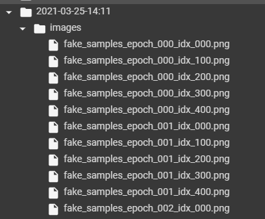
vutils.save_image 코드로 인해서, 다음과 같이 epoch과 batch index에 따라 다음과 같이 저장됨을 확인할 수 있습니다.
torch.save(netG.state_dict(), '%s/netG_epoch_%d.pth' % (weight_loc, epoch))
    torch.save(netD.state_dict(), '%s/netD_epoch_%d.pth' % (weight_loc, epoch))

    D_loss_epoch = torch.mean(torch.FloatTensor(D_losses))
    G_loss_epoch = torch.mean(torch.FloatTensor(G_losses))
    writer.add_scalars('Train/loss per epoch', {'Average Discriminator loss per epoch' : D_loss_epoch.item(),
                                 'Average Generator loss per epoch' : G_loss_epoch.item()}, epoch)
나머지 코드는 가중치 저장하고, loss를 계산하는 부분이니 넘어가겠습니다.
다른 논문 리뷰에서는 writer.add_scalar를 사용했는데, writer.add_scalars는 하나의 그림에 여러 개의 그림을 한 번에 그릴 때 씁니다. 즉, 그래프는 한 개지만 Discriminator loss와 generator loss를 다 표현하고 싶을 때 사용하는 것이죠.
맨 마지막에는 Summarywriter를 닫아줘야 하므로 writer.close()를 해줍니다.
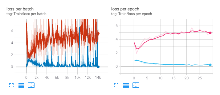
위 코드를 통해서 얻은 loss 그래프입니다. 왼쪽은 batch 별 loss, 오른쪽은 epoch 별 loss 입니다.
DCGAN을 통해서 만들어낸 이미지들을 가지고 gif로 만든 것입니다.
마지막으로, 논문에서 나왔던 latent space에 대해서 실험해본 내용을 보여드리고 마무리하도록 하겠습니다.
논문에서 6.1에 해당하는 부분인데요. latent space에서 interpolation을 진행해서 이미지가 어떻게 변하는지, sharp transition이 일어나는지 확인해본 내용입니다.
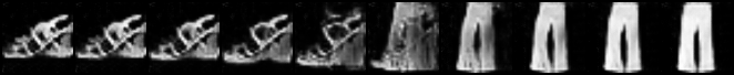
임의로 (1, 100) 짜리 Gaussian noise variable을 두 개 만든 뒤, 두 지점을 interpolation 해서 얻어낸 그림입니다.
왼쪽은 구두이고, 이것이 점점 변하면서 바지가 되는 모습을 볼 수 있습니다.
이는 Gaussian noise 값에 따라서 다른 모습들도 만들어낼 수 있습니다.

다른 random 값을 주어서, 다음과 같은 이미지도 얻을 수 있었습니다.
두 번째 이미지의 경우, 바지에서 상의로 변하는 모습을 볼 수 있습니다.
이렇게 점차적으로 변하는 모습을 확인할 수 있다면, 단순히 training image를 기억하는 것이 아닌 manifold를 학습했다고 보는 것 같습니다.
여기까지 해서 DCGAN 논문을 마무리 지으려고 합니다.
오늘 글에서 살펴본 모든 코드는 제 Github에서 확인하실 수 있습니다.
github.com/PeterKim1/paper_code_review
PeterKim1/paper_code_review
paper review with codes. Contribute to PeterKim1/paper_code_review development by creating an account on GitHub.
github.com
'(paper + code) review' 카테고리의 다른 글
| 5. Wasserstein GAN (WGAN) - code review (0) | 2021.04.16 |
|---|---|
| 5. Wasserstein GAN (WGAN) - paper review (0) | 2021.04.15 |
| 4. Unsupervised Representation learning with Deep Convolutional Generative Adversarial Networks(DCGAN) - paper review (0) | 2021.03.24 |
| 3. Adversarial Autoencoders(AAE) - code review (0) | 2021.03.22 |
| 3. Adversarial Autoencoders(AAE) - paper review (0) | 2021.03.21 |